Set

6- HOW TO SET THE PARAMETERS

Click here for command line version (Unix/DOS)

Windows 95/NT version: Menu

Toolbar:

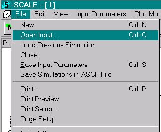
The parameters can be changed by
1) either opening an input file under the File menu:

2) using the button

on the toolbar.

or 3) by changing the values in the dialog box "Input Parameters".

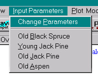
The dialog box can be accessed from the Input Parameters menu:

or by clicking the button

on the toolbar.

The model also has 4 defaults setting corresponding to 4 BOREAS southern study sites: Old Black Spruce, Young Jack Pine, Old Jack Pine, and Old Aspen.

The Input Parameters dialog box looks like this:

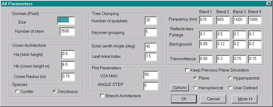
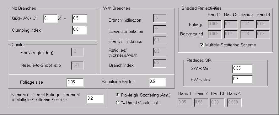
By pressing you will get the rest of the parameters:

See also Simple mode

The Parameters:

Domain (Pixel):

Size: we suggest 10000 m² for generic cases where the shaded proportions cannot be distinguished from the sunlit ones. Be careful when changing the size of the domain, the number of quadrats may need to be adjusted (see simple mode)

Number of stem: Enter the number of trees you have in the domain area

Tree Clumping:

Number of Quadrats: Divides the domain (pixel) into smaller area (quadrat). It also represents the maximum extend of a cluster of trees. You should be careful to make sure that the mean number of trees in a quadrat is less than about 200 (for computational reason). See Figs. 2 and 3 in [1] to understand the limitations of the model. The model should give you an error message if you choose too large or too small quadrats. Use the simple mode for an automatic calculation of the number of quadrats. Because of the elongation of the shadows with solar zenith angle, the size of the quadrat may need to be large enough to consider this, but has not been tested.

Neyman grouping:
Factor that distributes the trees in clusters. It is a double Poisson distribution process. Choosing "0" will produce the random case using the Poisson distribution. If you don't know what factor to use, we suggest a small number like 2 or 3.

Species

Conifer using the cone and cylinder shapes or
Deciduous using the spheroid shape.

Geometry of the crown

H_a: the stick
H_b: Cylinder height (for conifer),
or crown height (for deciduous)
r: Crown radius

Conifer

Needle-to-shoot ratio g_E

Used for taking into account the clumping of the conifer needles in shoots. Typical value: 1.40 (ranges from 1.20 to 2.10)

Black Spruce: 1.40
Jack Pine: 1.30-1.40
Red Pine: 2.07

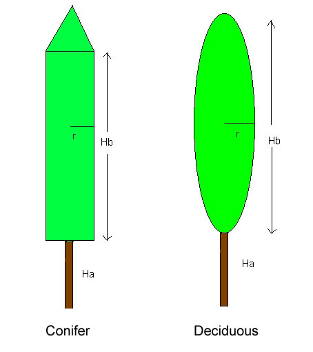
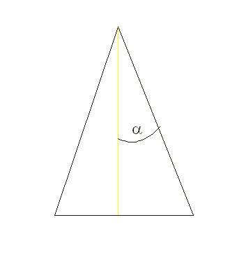
Half Apex Angle a

Angle of the cone part of the conifers. Can be estimated from photographs.

Without Branch Architecture

The clumping index W_E

It is the value measured in the forest stand (e.g., with TRAC). The model assumes that half of the forest clumping is due to having foliage in crowns, so the value used in equation (22) [1] is computed as W_{E
(in model)}= W_E
(input)+ (1 - W_E
(input)))/2_.When using the branch architecture, W_E is implicitly computed ( its value cannot be changed in the parameters dialog box of the Windows 95/NT version). Typical range: Grassland: 0.8-1.0
Deciduous: 0.6-0.9
Conifers: 0.5-0.8

Projection of unit leaf area G(q)

When not known, G(q) = 0.5 representing the random case is a good approximation for most canopies. Measurements of different canopies [12] show that G(q) is usually close to 0.5.
Empirical values for Douglas Fir stands [17]:

G(q) = 0.54 + 0.33q for q < 48.7° (0.85 radian)
G(q) = 0.82 - 1.14(q-0.85) for q > 48.7° (0.85 radian)

When using the branch architecture, G(q) is automatically computed by 5-Scale.

Branch Architecture

Detail in Leblanc et al., 1999
You will need to enter the branch architecture parameters in the "more" section of the dialog.

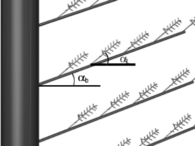Branch inclination a_b
Angle at which the branches are oriented from the horizontal.
Leaf orientation a_L
Angle at which the foliage (leaves or shoots)
is orientated from the horizontal.

Branch thickness: (in meters)

Ratio thickness/width for leaf: Important for conifers where the shoot is the foliage element since it has a thickness more important than a flat leaf.

Branch area index: typical 0.8-0.9

The typical element projection inside the crown (in metre). This parameter is used by the hotspot kernel.

Typical values:
Black Spruce: 0.03-0.04 m
Jack Pine:      0.05 -0.17 m (0.05 represents the shoots size, 0.17 represents the branches size)
Aspen:           0.02 - 0.10 m
Red Pine:       0.10-0.15 m
White Pine      0.05 m

LAI

The leaf area index of the canopy, defined as one half of the total foliage surface [9] per unit of ground surface.

Note that instruments like the LAI-2000 measure the effective LAI (Le).
The LAI is found from:

LAI = L_eg_E/W_E

There is no typical values given for LAI, but remember that the LAI is distributed in the number of trees you have. Adding trees will diminish the foliage density in each crown.

The woody material is not considered in this version of the model.

Reflectivities:

Foliage:

This is the reflectivities of the foliage (needles or leaves) in the Red (typically 0.05 to 0.15), Near Infrared (NIR) (typically 0.40 to 0.60) and Mid Infrared (MIR or SWIR).

Background:

Average reflectivity of the ground (background) under the canopy in the Red, Near Infrared (NIR) and Mid Infrared (MIR or SWIR). Boreal forests often have the following background: lichen, moss, different kinds of berries, etc.

Multiple Scattering:

Transmitance of the foliage:

Typical values: Red: 0.03-0.10 NIR:0.20-0.50

Diffused light:

Input the red (visible) value and the model with use reduced values for NIR and MIR bands, or use the Raleigh scattering approximation.

ANGLES:

Solar zenith angle (q_sor SZA) the model can handle SZA 0-80^o

Azimuth difference angle f: 0^o-360^o , but 360^o to 180^o is actually computed with 0^o to 180^o since symmetry is assumed
(i.e.,f = 1^ois the same as f=359^o )

VIEW ZENITH ANGLE (q_vor VZA) RANGE
The model is valid up to q_v = 80^o. Reflectance values can be computed for qv larger than 80^o, but with less accuracy.
The branch architecture is not giving a valid output at VZA=90^o.

VZA MAX is the maximum VZA of the plane.

PLOT STYLE output.

PLANE

Note that VZA = 0 is done twice (One with each f). The output has negative VZA corresponds to backscatering.

USER DEFINED

This option allows the user to vary different parameters (e.g., NDVI versus LAI, Individual bands versus SZA).

Example of User Defined file: SUN.UD3

HEMISPHERICAL

Used to reproduce '3D' plots like this:

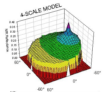This figure was produced with Sigma Plot by SPSS.

HYPERSPECTRAL

Used for hyperspectral reflectance at specific view and solar angles.

Fr controls the repulsion effect that forces branches from one tree to not overlap with branches in other trees.

Fr = 1 means maximum repulsion;
no overlap is allowed at nadir and
Fr = 0 means no repulsion;
the overlapping calculated by the negative binomial is allowed.

Comment line (up to 100-something characters; only UNIX in version)

Other parameters in .fs* files:

N_PHI 2 means that the next 2 lines contain phi angles.
For the reflectivities 1 = Red Reflectance
2 = Near Infrared
3 = Shortwave Infrared
G is the ground and T the tree crown.
Z is for shaded surfaces (not used in version 3.0).
f_B is used only if DIRECT is equal 1 (this may change to ON/OFF , or YES/NO in future versions)

Note that even when a values is not used, a default value needs to be in the file.

RUNNING 5-SCALE:

1) Enter the parameters (e.g., with the dialog box)
2) Press the RUN button (or Run model in the run menu)
3) While the model is running, this dialog appear and indicates the % done.

if "Cancel" is pressed, you get: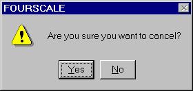

Allowing you to cancel the simulation.