BEPS-EASS is another version of BEPS, a coupled model with EASS. EASS(Ecosystem-Atmosphere Simulation Scheme) was developed
as a LSM based on remote sensing. The principle motivation
for formulating EASS is to provide realistic partition of
energy fluxes at regional scales as well as consistent estimates
of carbon assimilation rates. EASS has the following characteristics:
- satellite data are used to describe the spatial and temporal
information on vegetation;
- energy and water exchange and carbon assimilation in
soil-vegetation-atmosphere systems are fully coupled and
are simulated simultaneously;
- snow and soil simulations are emphasized by including
a flexible and multiple layer scheme.
EASS is based on a single vegetation canopy overlying a five-layer
soil, including physically based treatment of energy and moisture
fluxes from the vegetation canopy and through it. It also
incorporates explicit thermal separation of the vegetation
from the underlying ground. Similar to some former models
[e.g. Dickinson et al., 1986; Taconet et al.,1986; Tjernstrom,
1989], EASS treats the vegetation cover as a single layer
[Thom and Oliver, 1977] rather than lumping it together within
the ground. Moreover, EASS includes a scheme with stratification
of sunlit and shaded leaves to avoid shortcomings of the "big
leaf" assumption [de Pury and Farquhar, 1997; Liu et al.,
2003]. It has been referred as a "two-leaf" canopy model [Norman,
1980; Goudriaan, 1989; Chen and Coughenour, 1994; Chen et
al., 1999; Liu et al., 1997, 1999, 2002, 2003]. Canopy and
soil parameters, as model inputs, are derived from satellite
imagery and a database of soil textural properties [Shields
et al., 1991]. EASS follows and further develops the algorithms
embedded in FOREST-BGC [Running and Coughlan, 1988] to describe
the physical and biological processes in vegetation. With
spatially explicit input data on vegetation, meteorology and
soil, EASS can be run pixel by pixel over a defined domain,
such as Canada's landmass, or any of its parts, or the Globe.
Similar to BESP [Liu et al., 2003], it has flexible spatial
and temporal resolutions, as long as the input data of each
pixel are defined.
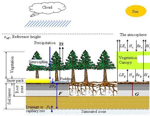
Figure1. The structure of
EASS model. Three components (soil, vegetation and the atmosphere)
are considered in EASS, which are integrated with two interfaces.
The right panel illustrated energy fluxes between these three
components. , , , , and are the latent heat flux, sensible
heat flux, shortwave radiation, longwave radiation, and soil
conductive heat flux, respectively; the subscripts g and c
present the energy fluxes at soil-canopy and canopy-atmosphere
interfaces, respectively. The left panel describes soil water
fluxes. The symbol F represents conductive water flux between
soil layers, and F0 represents the incoming water flux from
the surface to the top soil layer (i.e., the actual infiltration
rate ), and Fb is the water exchange (drainage or capillary
rise) between the bottom soil layer and the underground water.
The overall model structure is shown in Figure 1. We considered
the vertical profile of soil, vegetation (if present) and
the atmosphere as an integrated system with two interfaces.
Energy fluxes at canopy-atmosphere and soil-atmosphere (under
the canopy) interfaces can be summed to zero. The resulting
energy balance equations may be written in terms of mathmatical
descriptions of these fluxes. The water balances at these
interfaces are implicit in the energy balance equations. The
soil water balance equations are different from, but linked
to the surface energy balances. In EASS, the energy balance
and water balance are coupled, and both of them are discussed
separately at two levels: canopy and underlying ground (Figure
1). In compromise with limitations of available spatial data,
we assume that environmental and plant conditions are horizontally
uniform within a simulation unit (pixel) and lateral interactions
among pixels are neglectable. Thermal and moisture dynamics
therefore can be determined by vertical energy and water fluxes.
To accommodate using satellite data as model inputs, a single
vegetation layer is considered in EASS, and yet the multi-layer
scheme for energy exchanges and water transfers through the
soil profile and the snow pack (if present) is introduced
into EASS. The number of snow and soil layers and the depth
of each layer are user-defined according to soil physical
structures distributed in the profile, snow depth, and application
objectives and so forth. In the current study, the soil profile,
including forest floor (if it is forest), organic layers,
and mineral soil layers, is divided into seven layers and
the thickness of the layers increases exponentially from the
top layer to the sixth layer (equals to 0.05, 0.1, 0.2, 0.4,
0.8, 1.6m, respectively). The first 6 soil layers with a total
depth of 3.15 m are set to ensure the complete simulation
of energy dissipation in the soil column. The depth of the
last soil layer is adjusted according to water table depth.
Bottom boundary conditions are set to have a zero heat flux
and are free of drainage. The division of soil layers is applied
to the snow pack if present. The total depth of snow pack
is updated at every computing time step. When the thickness
of snow pack is thinner than 5 cm, it is treated as part of
the first soil layer and is weighted to obtain the grid cell
values. EASS was forced by near-surface weather variables
at a reference level zref within the atmospheric boundary
layer, including air temperature, relative humidity, in-coming
shortwave radiation, wind speed, and precipitation. The most
important time-invariant vegetation parameter is land cover
type as it is required in defining other parameters. These
parameters include vegetation height, canopy roughness length,
canopy zero plane displacement, standing mass, foliage clumping
index, leaf-angle distribution factor, ground roughness length,
and rooting depth, etc. The land cover type for each pixel
is identified as one of ten classes based on the original
31 classes in Cihlar et al. [1999]. The ten classes include
coniferous forest, mixed forest (mixture of coniferous and
deciduous forest), deciduous forest, shrub land, burned area,
barren land, cropland, grassland, urban area, and permanent
snow/ice area. The land cover map of Canada is generated to
provide an up-to-date, spatially and temporally consistent
national coverage. The data source is the Advanced Very High
Resolution Radiometer (AVHRR) onboard NOAA 14 satellite. Data
on soil texture (silt and clay fraction) are obtained from
the Soil Landscapes of Canada (SLC) database, the best soil
database currently available for the country [Shields et al.,
1991; Schut et al., 1994, Tarnocai, 1996; Lacelle, 1998].
The soil textural data for each EASS layer are directly from
SLC version 2.0. For soil depths where there are no default
data, the value of the layer immediately above it is used.
To generate these data layers with the same projection and
resolution as for other data layers, the original vector data
in SLC are mosaicked, reprojected and rasterized using the
ARC/INFO geographic information system [Chen et al., 2003].
Soil texture is crucial to soil properties, such as soil water
content at saturation (porosity), soil water potential at
saturation, soil heat and hydraulic conductivities at saturation,
etc. To determine the hydraulic and physical properties of
the soil layers, we classified soil texture into 11 categories
following Campbell and Norman [1998], Rawls et al. [1992],
and Kucharik et al. [2000]. Some of the time-varying vegetation
parameters, such as leaf area index, etc., are also generated
from satellite data using the algorithms developed by Chen
and Cihlar [1996] and Chen et al. [2002].
EASS was coupled with BEPS in recent years. The simulation
realism and accuracy in carbon dynamics were enhanced significantly
[Ju et al., 2004]. Test runs are conducted over Canada for
a week in August 2003. EASS is also tested and validated against
multiple-year observed data at several sites. Overall, EASS
is proved to be successful in capturing variations in energy
fluxes, canopy and soil temperatures, and soil moisture over
diurnal, synoptic, seasonal and inter-annual temporal scales.
|